 3 Dimensional Z-order Curve by Robert Dickau licensed under CC BY-SA 3.0
Part 1 of this series
3 Dimensional Z-order Curve by Robert Dickau licensed under CC BY-SA 3.0
Part 1 of this series
This second part of this series covering the K2 Graph, we'll see how to represent the graph as node genes and link genes. Then we'll see how the phenotype can be extracted and interpreted in a physical space.
Recall that genes in NEAT-like frameworks are of two types, node genes and link genes. The K2 Graph will be no different in that respect. What does change is the contents of the nodes and the structure of the links. Instead of containing a function, the nodes of the K2 Graph genome contain adjacency matrices. Furthermore, the K2 is a MultiDigraph, meaning that a pair of nodes can have multiple edges between them. Here's an example of a genome after 20 random mutations and k = 8.
Node Genes:
(1, {'constant': array([[ 0. ,  0. ,  0. ,  0. ,  0. ,  0. ,  0. ,  0. ],
       [ 0. ,  0. ,  0. ,  0. ,  0. ,  0. ,  0. ,  0. ],
       [ 0. ,  0. ,  0. ,  0. ,  0. ,  0. ,  0. ,  0. ],
       [ 0. ,  0. ,  0. ,  0. , -1.28323035,  0. ,  0.92546015,  0. ],
       [ 0. ,  0. ,  0. ,  0. ,  0. ,  0. ,  0. ,  0. ],
       [ 0. ,  0. ,  0. ,  0. ,  0. ,  0. ,  0. ,  0. ],
       [ 0. ,  0. , -0.88706943,  0.1605377 , -1.62884677,  0. ,  0. ,  0. ],
       [ 0. ,  0. ,  0. ,  0. ,  0.09582014,  0. ,  0.45323159,  0. ]])})
(2, {'constant': array([[ 0. ,  0. ,  0. ,  0. ,  0. , -0.03105544,  0. ,  0. ],
       [ 0. ,  0. ,  0. ,  0. ,  0. ,  0. ,  0. ,  0. ],
       [ 0. ,  0. ,  0. ,  0. ,  0. ,  0. ,  0. ,  0. ],
       [ 0. ,  0. ,  0. ,  0. ,  0.60063046,  0. ,  0. ,  0. ],
       [ 0. ,  1.37275931,  0. ,  0. ,  0. ,  0. ,  0. ,  0. ],
       [ 0. ,  0. ,  0. ,  0. ,  0. ,  0. ,  0. ,  0. ],
       [ 0. ,  0. ,  0. ,  0.1605377 , -1.62884677,  0. ,  0. ,  0. ],
       [ 0. ,  0. ,  0. ,  0. ,  0.09582014,  0. ,  0.45323159,  0. ]])})
(3, {'constant': array([[ 0. ,  0. ,  0. ,  0. ,  0. ,  0. ,  0. ,  0. ],
       [ 0. ,  0. ,  0. ,  0. ,  0. ,  0. ,  0. ,  0. ],
       [ 0. ,  0. ,  0. , -0.07005593,  0. ,  0. ,  0. ,  0. ],
       [ 0. ,  0. ,  0. ,  0. ,  0. ,  0. ,  0. ,  0. ],
       [ 0. ,  0. ,  0. ,  0. ,  0. ,  0. ,  0. ,  0. ],
       [ 0. ,  0. ,  0. ,  0. ,  0. ,  0. ,  0. ,  0. ],
       [ 0. ,  0. ,  0. ,  0.1605377 , -1.62884677,  0. ,  0. ,  0. ],
       [ 0. ,  0. ,  0. ,  0. ,  0.09582014,  0. ,  0.45323159,  0. ]])})
(4, {'constant': array([[ 0. ,   0. ,  0. ,  0. ,  0. ,  0. ,  0. ,  0. ],
       [ 0. ,  0. ,  0. ,  0. ,  0. , 0. ,  0. ,  0. ],
       [ 0. ,  0. ,  0. ,  0. ,  0. , 0. ,  0. ,  0. ],
       [ 0. ,  0. ,  0. ,  0. , -1.28323035,0. ,  0. ,  0. ],
       [ 0. ,  0. ,  0. ,  0. ,  0. , 0. ,  0. ,  0. ],
       [ 0. ,  0. ,  0. ,  0. ,  0. , 0. ,  0. ,  0. ],
       [ 0. ,  0. , -0.88706943,  0.1605377 ,  0. , 0. ,  0. ,  0. ],
       [ 0. ,  0. ,  0. ,  0. ,  0.09582014,  0. ,  0.45323159,  0. ]])})
Link Genes:
(1, 2, 26, {'weight': -1.9548930505912618, 'innovation': 1})
(1, 2, 51, {'weight': 0.34014684290296504, 'innovation': 6})
(1, 4, 41, {'weight': 1.0, 'innovation': 7})
(2, 3, 62, {'weight': 1.2949757677960567, 'innovation': 3})
The node genes consist of the node number followed by the internal matrix of the node. The link genes contain the parent node, the child node, and the parent node's element in the matrix that is linked to the child node, respectively
Previously we saw how an adjacency matrix can be extracted from the genome. Yet we have not placed the neurons represented in the adjacency matrix in any sort of physical space. How do we choose which nodes are inputs and which are outputs? Here's where space-filling curves, like the Z-order curve can help us.
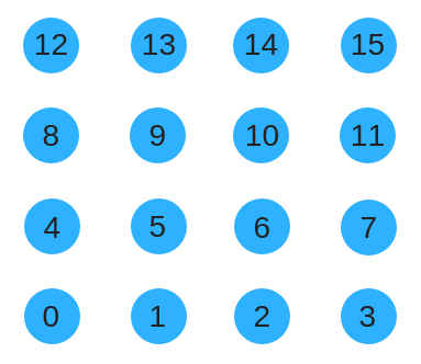
For a 2D substrate, we can arrange the nodes in a grid. To give a numbering to nodes we could try using row-col order like so.
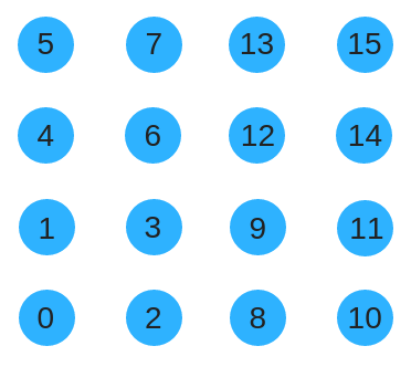
Unfortunately that wont work well because when the substrate grows genes will be encoding for completely different part of the grid. Instead, we could use a space filling curve such as the Z-order curve to renumber the substrate. This has the benefit of preserving locality as the substrate size grows. The same concept extends to higher spatial dimensions.
Say that now we wanted to give input to a neural network. First we map the nodes to evenly placed points on a Cartesian space, keeping the center of the grid at the origin. When the number of nodes increases they will occupy the same region but will become more densely packed. We also assign each of the inputs a location in this constructed Cartesian space. The input signals are then routed to the nearest neurons. As the neural network grows, the inputs stay in the same location but the neurons that receive the signal will change. For output, the output signal is queried from the nearest neurons to assigned output locations.
In the next post, we'll will create a simple experiment to evolve neural networks!