Hyperneat-adjacency-matrix

HyperNEAT is a well known Neuro-Evolution algorithm developed by Kenneth Stanley. HyperNEAT uses an indirect encoding called a Compositional Pattern Producing Network (CPPN) as the genotype. The CPPN is queried with substrate node coordinates to produce a connectivity pattern for the phenotype. This post will be analyzing the adjacency matrices that are produced when different space-filling curves are used to number the substrate nodes instead of ordering them by row-col order.

The reason for looking at the adjacency matrices of HyperNEAT in this way is to compare and contrast them to the adjacency matrices created by Compositional Adjacency Matrix Producing Networks (CAMPN). CAMPNs is an indirect encoding that directly produces an adjacency matrix without having to repeatedly query the genotype using coordinates. In fact, CAMPNs don't use spatial coordinates at all. Instead, substrate nodes are numbered using a space filling curve, which allows for locality to be preserved if the number of nodes in the substrate is to grow, as in ES-HyperNEAT. CAMPNs can be restricted from growing by limiting the number of Kronecker type nodes and in doing so, acts more like regular HyperNEAT where the substrate doesn't evolve.

If the theory behind CAMPNs is correct, a CAMPN should be able to produce a substrate resembling a HyperNEAT substrate. This is what I will be investigating.

In this post I'll be using Python Evolutionary Algorithms (https://github.com/noio/peas) produced by Thomas Van Der Berg.

Space Filling Curves

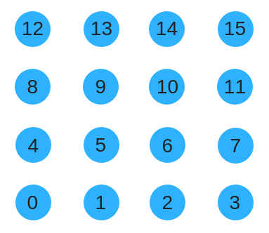
A CAMPN alone only produce an adjacency matrix but doesn't say which nodes are which within that matrix. To give an order to nodes we could try using row-col order like so.

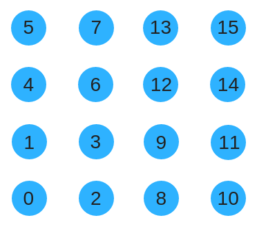
Instead, we could use a space filling curve such as the Z-order curve to renumber the substrate. This has the advantage of preserving locality as the substrate size grows.

The following code shows how to convert from a row-col ordering to Morton order. This is useful for converting from Cartesian coordinates

def unpart1by1(n):
    n &= 0x55555555
    n = (n ^ (n >> 1)) & 0x33333333
    n = (n ^ (n >> 2)) & 0x0f0f0f0f
    n = (n ^ (n >> 4)) & 0x00ff00ff
    n = (n ^ (n >> 8)) & 0x0000ffff
    return n


def deinterleave2(n):
    return unpart1by1(n >> 1), unpart1by1(n)

# Creates a mapping from row-col order to Z-order
map = {}
for i in range(0, 16):
    xpos, ypos = deinterleave2(i)
    map[ypos*4 + xpos] = i

I will also use a space filling curve I've been calling the Symmetric Z order curve. It looks like this.

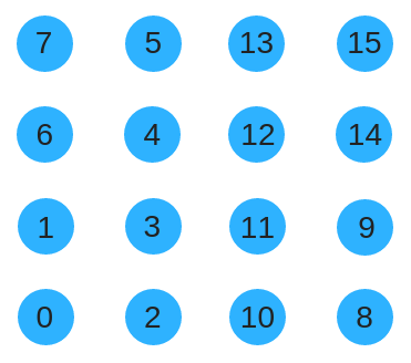
The Symmetric Z-order curve uses similar code to the Z-order curve but has a strange bit operator function that I've called "twirl" for lack of a better name. Note that the Symmetric Z-order curve can be generalized to a higher number of nodes just like the Z-order curve can.

def twirl(n):
    mask = 0x80000000

    for i in range(0, 15):
        n = n ^ ((n & (mask >> (2 * i + 1))) >> 1)
        n = n ^ ((n & (mask >> (2 * i))) >> 2)

    return n

map = {}
for i in range(0, 16):
    xpos, ypos = deinterleave2(twirl(i))
    map[ypos*4 + xpos] = i

HyperNEAT Adjacency Matrices

Now let's take a look at what an adjacency matrix for a Hyperneat substrate looks like.

HyperNEAT Adjacency Matrix

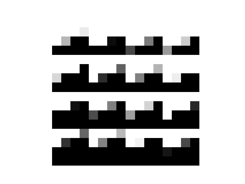
This is basically what all the HyperNEAT substrates looked like using peas.They appear a tiling of some motif with some variation. These type of patterns can easily be created with a Kronecker operation between two matrices. The left matrix will control the variation and the right matrix controls the appearance of the tile.

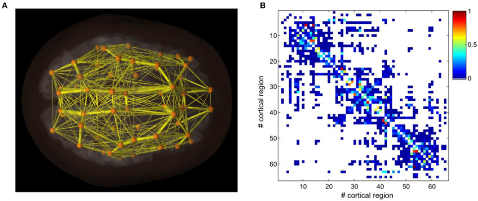
The reason why the Kronecker operation is interesting is because when a Z-order curve is used to order the adjacency matrix, the quadrants of the adjacency matrix appear similar to each other. It is very common for the top-left quadrant to be similar to the bottom-right quadrant and the top-right quadrant to be similar to the bottom-left quadrant for the adjacency matrices of actual brains. The reason is because the top-left and bottom-right quadrants contain all the connections within the left and right hemispheres, respectively. Whereas the top-right and bottom-left quadrants contain the interconnections between the hemispheres.

Also, as a side note -I didn't see any fracturing in the HyperNEAT substrates. Thomas Van Der Berg and Whiteson claimed that HyperNEAT had a difficult time in fractured domains (http://eplex.cs.ucf.edu/papers/stanley_ucftr13-05.pdf) but Stanley, Clune, and friends proved that Van Der Berg's hypothesis was wrong (http://eplex.cs.ucf.edu/papers/stanley_ucftr13-05.pdf). I am beginning to wonder if there is a problem with the peas implementation of HyperNEAT though I had a confused experience when trying to comb through the code.

Conclusion

These results make me hopeful for CAMPNs. If the HyperNEAT substrates can easily be created using a Kronecker operation it necessarily follows that CAMPNs can create similar substrates to CPPNs.

If you have any question or need clarification on something, don't hesitate to contact me at stefano.r.palmieri@gmail.com